SQL fundamentals

Lindsey Smith

The Data Manipulation Language (DML) component of SQL is used to interact with and manage the data stored in your tables. These statements form the core of regular SQL tasks and allow you to query, filter, and group your data.

On this page, we will focus on the following key statements and clauses:

• SELECT – to query data from a table
  • WHERE – to filter records based on conditions
  • ORDER BY – to sort results
  • GROUP BY – to group results and apply aggregate functions
  • JOIN – to combine rows from two or more tables based on common values in related columns

We won’t cover INSERT, UPDATE and DELETE statements today but you can view the syntax required for these operations by right clicking a table name in pgAdmin 4 and selecting Scripts.

Note on Literals

Before we start writing SQL statements, it’s important to note that different types of values (literals) require different formatting in order to be interpreted correctly:

• Text (i.e., string or non-numeric) values must be enclosed in single quotation marks
• Numeric values (e.g., integers, decimals) must not be enclosed in quotation marks
• Identifiers (e.g., table or column names) that contain spaces or special characters, or are case-sensitive should be enclosed in double quotation marks

For example:

INSERT INTO students(firstname, majorcode, group, "Dream Destination")
VALUES ('David', 2, 2, 'Spain');

SELECT Statement

The SELECT statement is perhaps the most commonly used SQL command. Its purpose is to retrieve and display data from one or more database tables. You can choose to return all fields, or just a subset of specific fields.

Every SELECT statement must include two mandatory clauses: - SELECT – specifies the fields (columns) you want to retrieve - FROM – specifies the table where the data is coming from

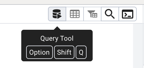
Access the database created in the Introduction to spatial databases tutorial. Within PgAdmin 4, open the Query tool.

PgAdmin Query Tool

We will check our data were imported correctly into the library visits table by executing the following query to retrieve all data.

Here, * is a wildcard which means ‘everything’. This is the simplest possible query to execute and returns all rows and fields from our data table.

SELECT * FROM visits;

We can also specify which fields to return which can be especially useful for tables with a large number of fields.

SELECT branchcode, visits FROM visits;

Once you’re comfortable retrieving data, you can start refining what you see in the output.

If your data, for example, has repeated values, the DISTINCT keyword allows you to return a list of unique values from the specified column. Any duplicates are automatically removed in the output.

For example:

SELECT DISTINCT branchcode FROM visits;

You can also control the order of your query results using the ORDER BY clause. By default, values are sorted in ascending (A–Z or lowest to highest) order. It’s also possible to switch to descending order using the DESC keyword, and to sort based on a number of fields.

For example: Sort in ascending order based on single field

SELECT * FROM visits
ORDER BY visits DESC;

For example: Sort with a mix of ascending/descending based on multiple fields

SELECT * FROM visits
ORDER BY branchcode, year DESC;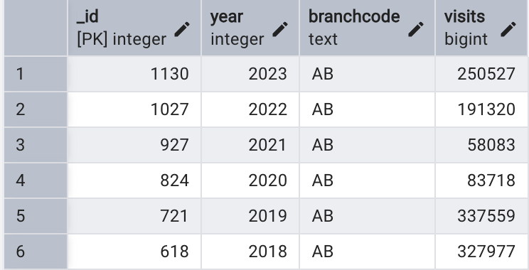

Query output: Rows sorted alphabetically by branchcode. For each branchcode, rows are ordered to list the most recent year first.

What we’ve covered here is just the beginning of what you can do with SELECT. These basics are intended to get you started, but there’s much more to explore including how to apply simple functions to create derived values (calculated on the fly as a query runs), and how to check for missing data using conditions. A few examples are shown below, but for a broader understanding of the full range of SQL functions and capabilities, you might also consider resources such as W3Schools or the PostgreSQL documentation.

-- Derived values
SELECT visits * 0.1, LEFT(branchcode, 1) FROM visits;

-- Checking for missing data
SELECT * FROM visits WHERE visits IS NULL;

WHERE Clause

Previous examples have returned all rows but often we need to restrict the rows that we receive from the data. The WHERE clause Limits the records included within the results depending on specified criteria. This is similar to the Select by Attribute option in ArcGIS Pro.

The criteria, or search expression, is evaluated as TRUE or FALSE for each row. WHERE may be used with a number of search expressions including comparisons, ranges, lists, patterns, and checks for missing values.

For example:

Type	Operators / Keywords	Example
Comparison	=, !=, <, >, <=, >=, NOT, AND, OR	WHERE visits > 50000
Range	BETWEEN, NOT BETWEEN	WHERE year BETWEEN 2018 AND 2020
Membership	IN, NOT IN	WHERE branchcode IN ('MA', 'BE')
Pattern Match	LIKE, NOT LIKE	WHERE branchcode LIKE 'H%'
Null Check	IS NULL, IS NOT NULL	WHERE visits IS NOT NULL

Below is an example query that will return all fields from the visits table for records where the branch code starts with the letter M and the year falls between 2020 to 2023. Results are ordered by year (most recent first) and then by highest number of visits:

SELECT * FROM visits
WHERE branchcode LIKE 'M%' AND year BETWEEN 2020 AND 2023
ORDER BY year DESC, visits DESC;

Now have a go at crafting your own complex search expressions!

Aggregate functions and the GROUP BY Clause

Aggregate functions are useful when you want to summarize values in a column, for example, to calculate totals, averages, or counts. These functions return a single result based on a single column and multiple rows.

Example aggregate functions:

Function	Description
COUNT()	Counts rows (can include or exclude duplicates)
SUM()	Adds up numeric values
AVG()	Calculates the average
MAX() / MIN()	Finds the highest or lowest value
STDDEV()	Returns standard deviation
VARIANCE()	Returns variance
CORR(a, b)	Correlation between two columns
COVAR(a, b)	Covariance between two columns

Example application of COUNT() function to data in visits table:

-- Count all rows in visits table
SELECT COUNT(*) FROM visits;

-- Count unique banch codes
SELECT COUNT(DISTINCT branchcode) FROM visits;

-- Count unique branch codes where over 50000 visits have been recorded
SELECT COUNT(DISTINCT branchcode) FROM visits
WHERE visits > 50000;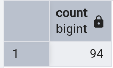

Single value returned from an aggregate function. In this case, 94 branches recorded more than 50000 in any year.

It’s also possible to use the GROUP BY clause to apply aggregate functions to subsets of your data. Here, aggregate results are grouped by a shared value.

For example, the following query sums the number of visits for each library branch code and orders the results alphabetically:

SELECT branchcode, SUM(visits) FROM visits
GROUP BY branchcode
ORDER BY branchcode;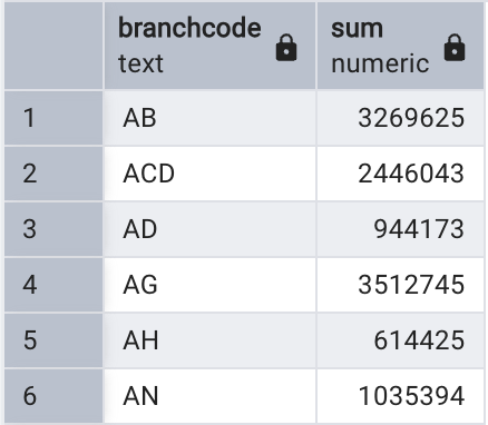

Single value returned for each unique branchcode, summing total visits across all years

Aliases

It’s possible to create aliases using the AS keyword (though this is actually optional and a space would work just fine, too).

Aliases let you rename a field or table in your query/output, making results easier to read or simplifying references to tables in complex queries. The latter is particularly useful when using queries to create JOINS which we will come to next.

In the example below we create: • Column aliases (branchcode AS branch, visits AS “Total Visits”) • A table alias (FROM visits AS v)

SELECT v.branchcode AS branch, v.visits AS "Total Visits"
FROM visits AS v;

While the table alias is not necessarily useful in this example, it gives you an idea of the syntax needed for more complex operations such as JOINS. If multiple tables have shared column names, the use of table aliases are important to avoid ambiguity across the tables.

JOINS

So far we have explored data within a single table. The real power of relational databases comes from the ability to use JOINs to combine rows of data from multiple tables based on shared values.

We will keep things relatively simple in this tutorial and focus on two types of JOINs:

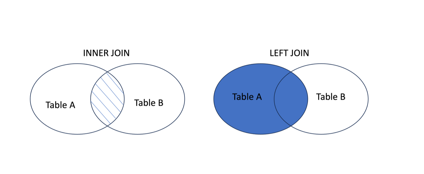
• INNER JOIN: Returns records where there is a matching value in table A and table B. Rows without a match are excluded from the results
• LEFT JOIN: returns all rows from table A (this is our left table as stated in the FROM cause) and includes matched data from table B (our right table as stated in the JOIN clause). This includes all rows from Table A in the results and where there’s no match in Table B, this will be shown as NULL

Inner and left table joins

Now let’s have a go at joining both our library visits and circulation tables. In the following example, both the year and branchcode are used to join the two tables since we want to join the annual circulation value for each branch.

SELECT v.branchcode, v.year, v.visits, c.circulation
FROM visits v
INNER JOIN circulation c
  ON v.branchcode = c.branchcode
  AND v.year = c.year;

Now that you’ve covered the fundamentals of SQL, you can start to think about how different clauses can come together to build more compex queries.

In the following example, we sum the total visits and circulation of materials for each branch in the year 2023, helping us identify the busiest libraries based on combined visitation and borrowing activity.

SELECT v.branchcode,
       SUM(v.visits + c.circulation) AS total_activity_2023
FROM visits v
INNER JOIN circulation c
  ON v.branchcode = c.branchcode
  AND v.year = c.year
WHERE v.year = 2023
GROUP BY v.branchcode
ORDER BY total_activity_2023 DESC;